💳 Handling Imbalanced Datasets: Fraud Detection Study Case

In my current research position, the project I am working on is related to financial fraud detection. In this particular domain, it is usual to have highly unbalanced data as the fraudulent transactions have a much lower volume than legitimate transactions.

To illustrate this scenario, I will use a dataset about credit card fraud detection to go over some common techniques to handle unbalanced datasets. It is a problem of imbalanced classification, and our task is to build a model to determine if a transaction is fraudulent or genuine.

Table of Contents:

1. Introduction
2. Dataset
3. Data Exploration
4. Data Preparation
5. Feature Engineering
6. Modelling
7. Conclusions

Introduction

The first thing to consider is the possible cause of the imbalance of the data, that can help narrow down which approaches we may use. As I mentioned before, in this example, imbalance is a characteristic of the problem domain. Before diving into the data, I will sum up a few strategies to handle imbalanced classification.

Is it possible to collect more data?

Collecting more data sometimes is overlooked. Evaluate whether it is possible to gather more data. If the size of the dataset is too small, it may not be representative enough of the context of the problem at hand. A larger dataset may be helpful in these situations and could provide more labelled examples of the minority class.

Resample the data

Try to even the balance of your data by resampling the dataset. There are two primary ways of achieving it:

1. Under-sampling, the idea is to remove examples of the majority class.
2. Over-sampling, add more data points of the minority class by creating copies of the existing examples or making similar ones.

There are still methods that combine the two approaches to try to overcome some individual disadvantages. For instance:

• Under-sampling may not work very well if the dataset is not big enough, as, after the sampling, we end up with very few data points.
• Over-sampling can be helpful when we don't have a lot of data. However, creating copies of the data points may not retain the original data distribution, features correlation and the underlying non-linear relationships.

Generate synthetic data

A simple way to generate synthetic data is to sample the attributes randomly from minority class examples. There are some systematic algorithms to do it. One of the most popular is the SMOTE algorithm. It creates new synthetic data points instead of copies of existing ones. It selects two or more similar examples (by a distance measure) and adds a random amount of noise to the attributes within the difference of their neighbours' data points.

Some more sophisticated methods involve using Deep Learning with Generative adversarial networks (GANs) to train a neural network that generates synthetic data to resemble the original data distribution.

Choose a more appropriate performance metric

When it comes to imbalanced classification, accuracy can be misleading and is not recommended to use it in this problem setting, there are some better alternatives.

Some options to consider:

• Precision, a measure of a classifier's exactness. The precision is intuitively the ability of the classifier not to label as positive a sample that is negative.
• Recall, a measure of a classifier's completeness. The recall is intuitively the ability of the classifier to find all the positive samples.
• F1 score, a weighted average of the precision and recall. The relative contribution of precision and recall to the F1 score are equal.
• Matthews correlation coefficient, a measure of the quality of binary and multi-class classifications. It takes into account all quadrants of the confusion matrix. It is generally regarded as a balanced measure that can be used even if the classes are very different.
• Precision-Recall Curve, the precision-recall curve, shows the tradeoff between precision and recall for different threshold. A high area under the curve represents both high recall and high precision.

Use different class weights or cost-sensitive models

Another possibility is to assign different weights to each label. In practice, we can specify a higher weight to the minority class during the model's training. We can also use versions of model algorithms that have penalised classification that impose an additional cost on the model for making classification mistakes on the minority class.

Frame the problem differently

Sometimes it helps to look at a problem from a different perspective. For example, we can think of an imbalance classification problem as an instance of anomaly detection. Anomaly detection is the detection of rare events. This change of perspective considers the minority class as the outliers class, which may help identify new ways to classify the data.

Dataset

The dataset I will use is called "Credit Card Fraud Detection", and it is available on Kaggle. The data was collected during a research collaboration of Worldline and the Machine Learning Group of ULB (Université Libre de Bruxelles) on big data mining and fraud detection. To describe the contents of the dataset, I will quote the original description:

The dataset contains transactions made by credit cards in September 2013 by European cardholders. This dataset presents transactions that occurred in two days, where we have 492 frauds out of 284,807 transactions. The dataset is highly unbalanced, the positive class (frauds) account for 0.172% of all transactions.

It contains only numerical input variables which are the result of a PCA transformation. Unfortunately, due to confidentiality issues, we cannot provide the original features and more background information about the data. Features V1, V2, … V28 are the principal components obtained with PCA, the only features which have not been transformed with PCA are 'Time' and 'Amount'. Feature 'Time' contains the seconds elapsed between each transaction and the first transaction in the dataset. The feature 'Amount' is the transaction Amount, this feature can be used for example-dependant cost-sensitive learning. Feature 'Class' is the response variable and it takes value 1 in case of fraud and 0 otherwise.

Data Exploration

We will start by setting a seed number to ensure the reproducibility of the results and then load the data into memory.

# Set seed for reproducibility
SEED = 1
random.seed(SEED)
np.random.seed(SEED)
os.environ['PYTHONHASHSEED'] = str(SEED)

We will define a customised read_csv method to optimise data types and use less memory.

def read_csv(file_path: str, nrows=None, dtype=np.float32) -> pd.DataFrame:
  with open(file_path, 'r') as f:
    column_names = next(csv.reader(f))
  dtypes = {x: dtype for x in column_names if x != 'Class'}
  dtypes['Class'] = np.int8
  return pd.read_csv(file_path, nrows=nrows, dtype=dtypes)

df = read_csv('/kaggle/input/creditcardfraud/creditcard.csv')
df.info()

This dataset does not contain missing values. Therefore we will proceed to make some data visualisations.

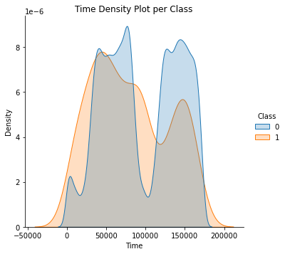
What is the distribution of the Time of the Transactions?
Remember that in this dataset, Time represents the seconds elapsed between transactions.

# We will use a copy of the DataFrame to make modifications for visualisation purposes only.
df_copy = df.copy()

ax = sns.displot(df_copy, x='Time', hue='Class', kind='kde', fill=True, common_norm=False)
ax.set(title='Time Density Plot per Class')

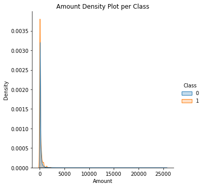
What is the distribution of Transactions' Amount?

ax = sns.displot(df_copy, x='Amount', hue='Class', kind='kde', fill=True, common_norm=False)
ax.set(title='Amount Density Plot per Class')

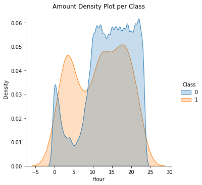
What is the distribution of Transactions' Amount, per hour of the day?

df_copy['Hour'] = df_copy['Time'].apply(lambda x: np.ceil(x / 3600) % 24)

ax = sns.displot(df_copy, x='Hour', hue='Class', kind='kde', fill=True, common_norm=False)
ax.set(title='Amount Density Plot per Class')

Next, we will compute some statistical data about our dataset.

tmp = df_copy.groupby(['Hour', 'Class'])['Amount'].aggregate(['min', 'max', 'count', 'sum', 'mean', 'median', 'var']).reset_index()
stats = pd.DataFrame(tmp)
stats.columns = ['Hour', 'Class', 'Min', 'Max', 'Transactions', 'Sum', 'Mean', 'Median', 'Var']

What is the volume of Transactions per hour of the day?
When we plot the volume of transactions per class grouped by hour of the day, we can observe some interesting patterns as fraud transactions seem to have spikes at specific hours and occur during typical sleeping hours.

fig, ax = plt.subplots(1,2, figsize=(12,5))
sns.lineplot(x='Hour', y='Transactions', data=stats.query('Class == 0'), ax=ax[0])
sns.lineplot(x='Hour', y='Transactions', data=stats.query('Class == 1'), color='red', ax=ax[1])
fig.suptitle('Total Number of Transactions per Hour of the Day')
ax[0].set(title='Legit Transactions')
ax[1].set(title='Fraud Transactions')
fig.show()

Data Preparation

To build the model, I incrementally increased the fraction of data used by 20% to adjust the model parameters progressively to avoid overfitting. For this final build, we will use the entirety of the dataset.

df = df.sample(frac=1, random_state=SEED).reset_index(drop=True)

y = df['Class']
X = df.drop('Class', axis=1)

feature_names = X.columns.tolist()

For the train/test split, we will divide them into 80% for the train data and 20% for the test data in a stratified fashion.

X_train, X_test, y_train, y_test = train_test_split(X, y, test_size=0.2, stratify=y, shuffle=True, random_state=SEED)

Feature Engineering

We will compute some additional features containing statistical information about the anonymised variables.

def get_group_stats(df: pd.DataFrame) -> pd.DataFrame:
  """
  Create features by calculating statistical moments.
  
  :param df: Pandas DataFrame containing all features
  """
  cols = list(filter(lambda x: x.startswith('V'), df.columns))
  
  # avoid warnings about returning-a-view-versus-a-copy
  ds = df.copy()
  
  ds['V_mean'] = df[cols].mean(axis=1)
  ds['V_std'] = df[cols].std(axis=1)
  ds['V_skew'] = df[cols].skew(axis=1)
  
  return ds

X_train = get_group_stats(X_train)
X_test = get_group_stats(X_test)

We will train our model using cross-validation. To generate the splits, we will be applying a GroupKFold strategy. The group will be based on the hour of the day of the given transaction. From a previous plot, we could observe that specific hours have a higher volume of fraudulent transactions.

# Tested stratified kfold as well
sfold = StratifiedKFold(n_splits=3)

hour_train = X_train['Time'].apply(lambda x: np.ceil(float(x) / 3600) % 24)

gfold = GroupKFold(n_splits=3)
groups = list(gfold.split(X_train, y_train, groups=hour_train))

def plot_correlation(corr: str) -> plt.Axes:
  mask = np.triu(np.ones_like(corr, dtype=bool))
  f, ax = plt.subplots(figsize=(11, 9))
  cmap = sns.diverging_palette(230, 20, as_cmap=True)
  sns.heatmap(corr, mask=mask, cmap=cmap, vmax=.3, center=0,
              square=True, linewidths=.5, cbar_kws={"shrink": .5})

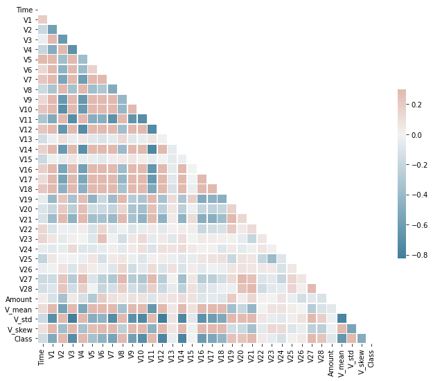
plot_correlation(X_train.corr(method='spearman'))

It is also good practice to look at features correlation as it may help recognise which features could have a more significant predictive factor.

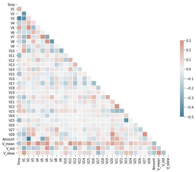
Because the data is highly unbalanced, it isn't easy to see the correlation between some features. However, after experimenting with undersampling the data to reduce the number of examples of the majority class (legit transactions) and have equal class proportions, we can now see that the correlation values are more noticeable. We will use the correlation amount to select higher correlated features with our target class.

sampler = RandomUnderSampler(random_state=SEED)
X_resampled, y_resampled = sampler.fit_resample(X_train, y_train)
X_resampled['Class'] = y_resampled

plot_correlation(X_resampled.corr(method='spearman'))

We will select features that have a correlation with our target class higher than the lower quartile value. Dropping features with low correlation can help to reduce the complexity of the model.

def select_features_correlation(df: pd.DataFrame) -> list:
  # Calculate correlations with target
  full_corr = df.corr(method='spearman')
  corr_with_target = full_corr['Class'].T.apply(abs).sort_values(ascending=False)
  
  min_threshold = corr_with_target.quantile(.25)
  
  # Select features with highest correlation to the target variable
  features_correlation = corr_with_target[corr_with_target >= min_threshold]
  features_correlation.drop('Class', inplace=True)
  return features_correlation.index.tolist()

cols = select_features_correlation(X_resampled)
X_train = X_train[cols]
X_test = X_test[cols]

Modelling

We will make a baseline model and then use hyperparameter optimisation for tuning the final model. And, we will apply cross-validation using the group fold strategy as mentioned above. To evaluate the performance:

• We will use the F1-score, a more relevant metric in this situation, since false positives and false negatives are both critical.
• We will use a maximum depth value to prevent overfitting the training data.
• We will test using different percentages of features used by each tree.
• Finally, we will try out two possibilities for the learning rate.
• I kept other parameters to fine-tune the alpha regularisation value and the subsample of the training set for future changes.

Baseline

First, we will train a simple baseline model with default parameters to have some initials results that we can compare with and identify what things we aim to improve.

pipeline = Pipeline([
  ('standardscaler', StandardScaler()),
  ('clf', LGBMClassifier(n_jobs=-1, random_state=SEED)),
])

mcc_results = []
ap_results = []
roc_auc_results = []
f1_results = []

for train_index, test_index in groups:
  pipeline.fit(X_train.values[train_index], y_train.values[train_index])
  test_data = pipeline['standardscaler'].transform(X_train.values[test_index])
  
  y_pred = pipeline.predict(test_data)
  
  mcc_results.append(matthews_corrcoef(y_train.values[test_index], y_pred))
  ap_results.append(average_precision_score(y_train.values[test_index], y_pred))
  roc_auc_results.append(roc_auc_score(y_train.values[test_index], y_pred))
  f1_results.append(f1_score(y_train.values[test_index], y_pred))

print(f'Baseline MCC score: {np.mean(mcc_results)}')
print(f'Baseline AP score: {np.mean(ap_results)}')
print(f'Baseline ROC AUC score: {np.mean(roc_auc_results)}')
print(f'Baseline F1 score: {np.mean(f1_results)}')

# Baseline MCC score: 0.23349372444054892
# Baseline AP score: 0.08047800670729233
# Baseline ROC AUC score: 0.7221486689515286
# Baseline F1 score: 0.2026884752773078

Our baseline model does not perform great. We can establish that it still does better than a random guess. Still is essential to mention that its performance can change slightly using different seed values. This code is just for demonstration purposes, and in a production environment, this needs to be tested more thoroughly with various trials to average the results.

Fine-Tuning with Grid Search

To improve our baseline model, we will perform a grid search to fine-tune the model parameters using cross-validation. To evaluate the performance of the cross-validated model on the test set, we will use the F1 score.

gbm_grid = {
  'clf__n_estimators': [500, 1000],
  'clf__learning_rate': [0.1, 0.01],
  'clf__max_depth': [4, 6, 8],
  'clf__colsample_bytree': np.linspace(0.6, 1.0, num=5),
  # 'clf__reg_alpha': np.linspace(0., 1.0, num=5),
  # 'clf__subsample': np.linspace(0.7, 1.0, num=4),
}

def grid_search_tuning(pipeline, X, y, grid, fold):
  grid = HalvingGridSearchCV(pipeline, param_grid=grid, cv=fold, scoring='f1',
                              random_state=SEED, n_jobs=-1, verbose=1)
  grid.fit(X, y)
  
  print(f"\nMean test score: {np.mean(grid.cv_results_['mean_test_score'])}")
  print(f'Best parameters: {grid.best_params_}')
  
  return grid.best_estimator_

pipeline = Pipeline([
  ('standardscaler', StandardScaler()),
  ('clf', LGBMClassifier(n_jobs=-1, random_state=SEED)),
])

# It can take a while to run
grid = grid_search_tuning(pipeline, X_train, y_train, gbm_grid, groups)

Next, we define a helper function to score our model and plot some additional metrics and feature importance.

def score_model(clf, X_test, y_test, feature_names):
  y_pred = clf.predict(X_test)
  y_probas = clf.predict_proba(X_test)

  print(classification_report_imbalanced(y_test, y_pred, target_names=['Legit', 'Fraud']))
  print(f'MCC: {matthews_corrcoef(y_test, y_pred)}\nAP: ' +
        f'{average_precision_score(y_test, y_pred)}\nROC AUC: {roc_auc_score(y_test, y_pred)}')

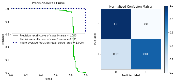
  fig, ax = plt.subplots(1,2, figsize=(12,5))
  skplt.metrics.plot_precision_recall(y_test, y_probas, ax=ax[0])
  skplt.metrics.plot_confusion_matrix(y_test, y_pred, normalize=True, ax=ax[1])
  fig.show()
  
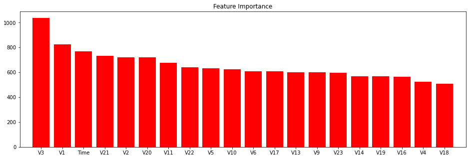
  skplt.estimators.plot_feature_importances(clf, feature_names=feature_names, figsize=(16,5))

  return y_probas

scaled_X_test = grid['standardscaler'].transform(X_test)
y_probas = score_model(grid['clf'], scaled_X_test, y_test, feature_names)

                   pre       rec       spe        f1       geo       iba       sup

      Legit       1.00      1.00      0.81      1.00      0.90      0.82     56864
      Fraud       0.95      0.81      1.00      0.87      0.90      0.79        98

avg / total       1.00      1.00      0.81      1.00      0.90      0.82     56962

MCC: 0.8757493736676086
AP: 0.7676067300337754
ROC AUC: 0.9030260528522045

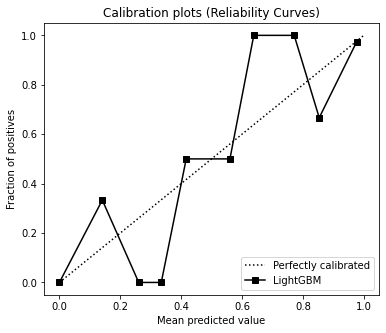
skplt.metrics.plot_calibration_curve(y_test, [y_probas], ['LightGBM'], figsize=(6,5))

Finally, we will look at two more plots:

• The calibration curve helps determine whether or not you can interpret their predicted probabilities directly as a confidence level.
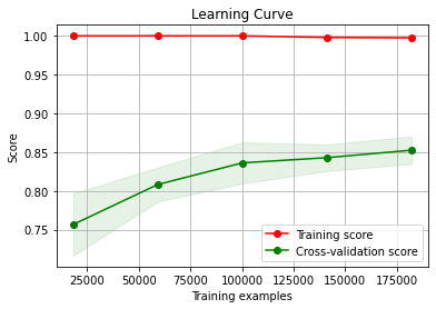
• The learning curve helps diagnose whether the model is overfitting or underfitting the training data and, with the validation data, gives an idea of how well the model is generalising.

skplt.estimators.plot_learning_curve(grid['clf'], X_train, y_train,
                                     scoring='f1', n_jobs=-1, random_state=SEED)

Conclusions

With this dataset, resampling the data didn't produce good results. Using under-sampling, over-sampling or a combination of both didn't improve compared with unchanged class proportions. Perhaps, since most variables were from a PCA transformation, that affected the impact of sampling. Another potential reason is the low number of fraudulent examples caused the under-sampling to produce a tiny dataset, lacking enough data to train a decent model.

In a fraud detection system, two cases are essential for a successful solution: achieving the primary goal of detecting fraudulent transactions (true positive examples) and avoiding targeting genuine transactions as fraudulent (false positives). These two are the most costly to a business when the system does not perform well. This model delivers good results at identifying true positives with an F1 score of 0.87 and does not label any genuine transactions as fraudulent.

You can check the complete code for this project in this repository.

Thank you for taking the time to read. You can follow me on Twitter, where I share my learning journey. I talk about Data Science, Machine Learning, among other topics I am interested in.