🚢 Predicting the Outcome of the Titanic Passengers
The Kaggle's Titanic Competition is a well-known beginner's Machine Learning problem. The goal is simple: Using Machine Learning create a model to predict which passengers survived the shipwreck.
This is a good starting point to build a complete first project. And have the opportunity to explore different techniques along the way.
In this post, I would like to share some of the ideas I have applied to tackle this project and guide you through the different steps of the work done.
I will begin doing some data exploration and visualization. To get a better understanding of the dataset. The next step is to handle any missing values and perform feature engineering to extract some new insights from the data. Finally, I will try to predict the outcome using different models and compare their performances to find the most suitable one for this project. In the end, I will attempt to improve the results by optimizing the final model parameters.
Table of Contents:
- Installing Dependencies and Importing Libraries
- Exploring the Data
- Data Cleaning
- Creating and Training the Models
- Fine-Tuning and Additional Improvements
- Predicting the Outcome
- Final Thoughts
Installing Dependencies and Importing Libraries
Before diving into the project, make sure you have these requirements installed:
- Python 3 (at the time of writing, I am using Python 3.7.10)
- SciPy (which includes NumPy, SciPy, Pandas, IPython, and matplotlib)
- scikit-learn
- Seaborn
Then, we will import the necessary packages:
import re
import numpy as np
import pandas as pd
import matplotlib.pyplot as plt
import seaborn as sns

from scipy.stats import zscore

from xgboost import XGBClassifier

from sklearn.svm import SVC
from sklearn.ensemble import RandomForestClassifier
from sklearn.tree import DecisionTreeClassifier
from sklearn.linear_model import LogisticRegression
from sklearn.neighbors import KNeighborsClassifier
from sklearn.neural_network import MLPClassifier

from sklearn.metrics import (classification_report, plot_confusion_matrix,
                             roc_auc_score, matthews_corrcoef)
from sklearn.model_selection import (GridSearchCV, cross_validate,
                                     cross_val_score, cross_val_predict,
                                     train_test_split, KFold)
Exploring the Data
We will start by loading the train and test data and taking a peek at the first rows and data summary:
train_data = pd.read_csv('train.csv')
test_data = pd.read_csv('test.csv')
train_data.info()
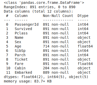
We can observe that the training data has 891 examples and 11 features plus the target class (survived). Seven of the features are numerical, while 4 are categorical.
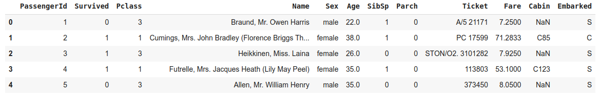
train_data.head()
Next, we need to know what each column of our dataset represents and what values they can have. Here is a description, taken from the Kaggle competition:
| Variable | Definition | Key |
|---|---|---|
| survival | Survival | 0 = No, 1 = Yes |
| pclass | Ticket class | 1 = 1st, 2 = 2nd, 3 = 3rd |
| sex | Sex | |
| Age | Age in years | |
| sibsp | # of siblings / spouses aboard the Titanic | |
| parch | # of parents / children aboard the Titanic | |
| ticket | Ticket number | |
| fare | Passenger fare | |
| cabin | Cabin number | |
| embarked | Port of Embarkation | C = Cherbourg, Q = Queenstown, S = Southampton |
We can look further at some features. Inspecting their data distributions and asking some questions.
# List of features to view descriptive statistics
features = ['Pclass', 'Name', 'Sex', 'Age', 'SibSp',
'Parch', 'Ticket', 'Fare', 'Cabin', 'Embarked']
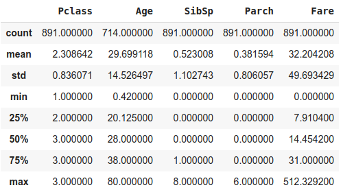
train_data[features].describe(include=[np.number])
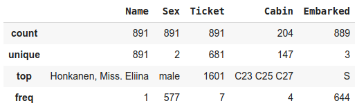
train_data[features].describe(exclude=[np.number])
Is our training data balanced? Do we have a reasonable distribution of passengers who survived and those who did not?
The training data is reasonably balanced. Around 61% of the passengers died, and approximately 38% survived.
train_data['Survived'].value_counts(normalize=True)
# 0    0.616162
# 1    0.383838
# Name: Survived, dtype: float64
Do we have missing values in our training data and/or testing data?
We have some missing values in both training and testing sets. We will come back to it later on.
train_data.isna().sum()
# PassengerId      0
# Survived         0
# Pclass           0
# Name             0
# Sex              0
# Age            177
# SibSp            0
# Parch            0
# Ticket           0
# Fare             0
# Cabin          687
# Embarked         2
# dtype: int64
test_data.isna().sum()
# PassengerId      0
# Pclass           0
# Name             0
# Sex              0
# Age             86
# SibSp            0
# Parch            0
# Ticket           0
# Fare             1
# Cabin          327
# Embarked         0
# dtype: int64
Data Visualization
Creating data visualizations can make it easier to spot data patterns. We will ask a few more questions about the data, looking at different plots. This can give us insights into how the features are related to each other. And which ones could have a higher impact on the survival rate of the passengers.
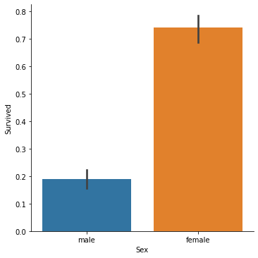
Did one gender survive more than the other?
We can confirm that a significantly higher percentage of female passengers survived compared to the male passengers.
sns.catplot(x='Sex', y='Survived', kind='bar', data=train_data)
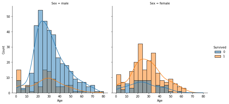
What is the distribution of passengers ages, which Age groups had higher survival odds, comparing gender?
The passengers' ages seem to follow a normal distribution.
sns.displot(x='Age', hue='Survived', col='Sex', kde=True, data=train_data)
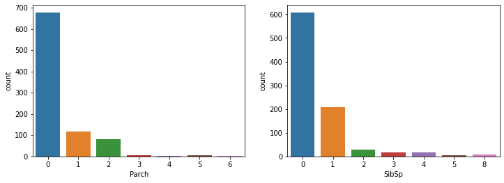
What is the distribution of passengers parents/children and siblings/spouses aboard?
The majority of passengers travelled alone or with small families/groups. However, a few groups of passengers were quite large, close to ten people.
fig, ax = plt.subplots(1,2, figsize=(12,4))
sns.countplot(x='Parch', data=train_data, ax=ax[0])
sns.countplot(x='SibSp', data=train_data, ax=ax[1])
fig.show()
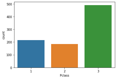
What is the distribution of passengers per ticket class?
Most passengers were from the 3rd class. While the least number of passengers were from 2nd class.
sns.countplot(data=train_data, x='Pclass')
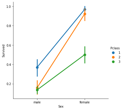
Which classes of passengers survived the most? Comparing gender.
It seems that passengers with higher classes had a better survival rate overall. When comparing gender, the difference is more pronounced with the female passengers of the upper classes, having a much higher survival rate than the male passengers. Also, female passengers of the upper classes survived more than the female passengers of the 3rd ticket class.
sns.catplot(x='Sex', y='Survived', hue='Pclass', kind='point', data=train_data)
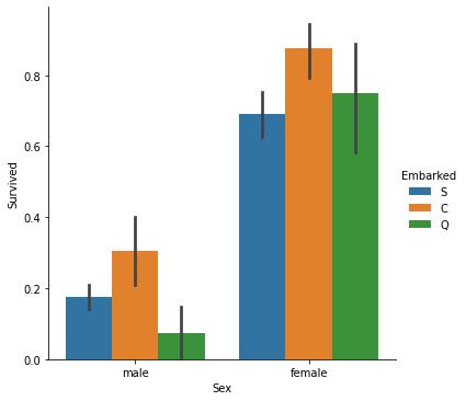
Which places of embarking have the most survivors? Comparing gender?
Passengers from Cherbourg (C), both men and women, had a higher survival rate than the other two cities.
sns.catplot(x='Sex', y='Survived', hue='Embarked', kind='bar', data=train_data)
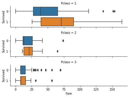
What is the likelihood of survival by Fare price? Comparing passenger classes?
Passengers who paid for more expensive tickets had higher survival rates. Naturally, the group with more passengers with expensive tickets were from the 1st class.
sns.catplot(x='Fare', y='Survived', row='Pclass', kind='box',
            orient='h', height=1.5, aspect=4, data=train_data)
Data Cleaning
Removing Outliers
After looking at the data, the Fare feature displays some potential outliers values. One plot that can help visualize them is a box-and-whisker plot:
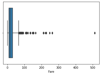
In this plot, points are determined to be outliers using a method that is a function of the inter-quartile range. However, we will use a different approach to identify the outliers by calculating the z-score and removing entries with z-score with absolute values higher than 3.
fare_outliers = train_data[np.abs(zscore(train_data['Fare'])) > 3]
train_data = train_data.drop(fare_outliers.index).reset_index(drop=True)
Handling Missing Values
As we saw before, there are a total of 4 features containing missing values: Cabin, Age, Embarked and Fare.
Age
For the feature Age, I have seen people approaching it in a few ways: Some prefer to group the Age in a certain number of bins. There are some examples where they train a regressor model to predict the missing values. Another way, which is the one I am adopting, is to create a normal distribution based on the existing values to fill in the missing ones. I will define a function to generate the Age distribution and fill in the missing values on the train and test data sets:
def age_dist(df):
  mean = np.mean(df['Age'])
  std = np.std(df['Age'])
  return np.random.randint(mean - std, mean + std, size=df['Age'].isna().sum())

train_data.loc[train_data['Age'].isna(), 'Age'] = age_dist(train_data)
test_data.loc[test_data['Age'].isna(), 'Age'] = age_dist(test_data)
Embarked
There are only two data points with missing values for the feature Embarked on the train data set. After searching for the passengers' names, I found records showing that they boarded the Titanic from Southampton.
train_data.loc[:, 'Embarked'] = train_data['Embarked'].fillna('S')
Fare
In regards to the Fare feature, there is just one entry with missing information. To fill in the missing Fare value, we will look at the median fare cost for this specific passenger class and the same family size.
median = test_data.query('Pclass == 3 & SibSp == 0 & Parch == 0')['Fare'].median()
test_data.loc[test_data['Fare'].isna(), 'Fare'] = median
Cabin
The Cabin feature is more difficult to deal with since a large portion of the values is missing. To understand better how cabins were organized on the Titanic, let us take a look at the following blueprint:
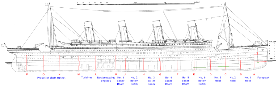
We can't simply ignore this feature, as some cabins may have higher survival rates. As we can see from the blueprint image, the first letter of the Cabin values are the decks where they were located. Those decks were, for the most part separating passenger classes. Still, a few of them were shared by multiple passenger classes.
- Decks A, B and C were reserved for 1st class passengers.
- Decks D and E had passengers from all classes.
- Decks F and G had passengers from 2nd and 3rd classes.
- Moving from Deck A to G, the distance from the staircase increases, which may impact survival rates.
- There is only one passenger on Deck T who was first class. He will be grouped with Deck A since it has the most resemblance with their passengers.
- Passengers with missing values for Cabin will be labelled with Deck M.
for df in [train_data, test_data]:
  df.loc[df['Cabin'] == 'T', 'Cabin'] = 'A'
  df['Deck'] = df['Cabin'].apply(lambda x: x[0] if pd.notna(x) else 'M')
  df['Deck'] = df['Deck'].fillna('M')
Applying Feature Engineering
In this section, I will create new features to extract more information about the data. And do feature transformation by converting and encoding some values to numerical types.
Extracting New Features
Title
From the passengers' name information, we can infer data about their social status. I will define a function to extract the Title information and group less common values together. This feature will complement the passenger class information.
def get_title(name):
    title_search = re.search(' ([A-Za-z]+)\.', name)
    # If the title exists, extract and return it.
    if title_search:
        return title_search.group(1)
    return ''

for df in [train_data, test_data]:
  df['Title'] = df['Name'].apply(get_title)

  df['Title'] = df['Title'].replace(['Lady', 'Countess','Capt', 'Col','Don', 'Dr', 'Major', 'Rev', 'Sir', 'Jonkheer', 'Dona'], 'Rare')
  df['Title'] = df['Title'].replace('Mlle', 'Miss')
  df['Title'] = df['Title'].replace('Ms', 'Miss')
  df['Title'] = df['Title'].replace('Mme', 'Mrs')
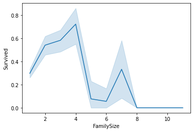
Family Size
We can sum features SibSp and Parch plus one to represent the passenger himself, to get the Family Size of a given passenger. We can observe that less numerous families had higher survival rates. At the same time, there is a curious fact where families around seven people had a spike in survival rate.
for df in [train_data, test_data]:
  df['FamilySize'] = df['SibSp'] + df['Parch'] + 1

sns.lineplot(x='FamilySize', y='Survived', data=train_data)
Encoding Features and Removing unused ones
First, we will convert the Deck letter value into its integer representation using the function ord. Next, we will perform one-hot encoding for the features Sex, Pclass, Embarked and Title.
for df in [train_data, test_data]:
  df['Deck'] = df['Deck'].apply(ord)

train_data = pd.get_dummies(train_data, columns=['Sex', 'Pclass', 'Embarked', 'Title'])
test_data = pd.get_dummies(test_data, columns=['Sex', 'Pclass', 'Embarked', 'Title'])
Finally, we discard some features that are no longer necessary. Either were transformed or are not relevant to our modelling step.
drop_elements = ['PassengerId', 'Name', 'Ticket', 'Cabin', 'Surname']

train_data = train_data.drop(drop_elements, axis=1)
test_data = test_data.drop(drop_elements, axis=1)
Creating and Training the Models
Before defining the models, we will separate the features and the labels into the variables X and y, respectively. And keep some variables about the metadata of our dataset. To evaluate the models' performance, we will use the following metrics:
- Compute Area Under the Receiver Operating Characteristic Curve (ROC AUC)
- Matthews Correlation Coefficient (MCC)
X = train_data.drop('Survived', axis=1)
y = train_data['Survived']
X_test = test_data.copy()

feature_names = X.columns.to_list()
num_features = X.shape[1]
Next, we will set our cross-validation strategy and create a data frame to hold our models' scores. We will also create a scaler object to standardize our data. It is also crucial to define a seed number to ensure that our model workflow is reproducible.
Standardization of a dataset is a common requirement for many machine learning estimators. They might behave unexpectedly if the individual features do not more or less look like standard normally distributed data. -- Source: scikit-learn
seed = 42
np.random.seed(seed)
kfold = KFold(n_splits=10, shuffle=True, random_state=seed)
standard_scaler = StandardScaler()
model_results = pd.DataFrame(columns=['Model', 'Train Score', 'Val Score', 'MCC'])
We will create a helper function to train each model and evaluate the training score with cross-validation using a ten-fold split.
def model_algorithm(clf, name, X_train, y_train, X_validate, y_validate):
  cv_results = cross_validate(clf, X_train, y_train, cv=kfold,
                              scoring='roc_auc',
                              return_estimator=True)

  clf = cv_results['estimator'][np.argmax(cv_results['test_score'])]

  y_probas = clf.predict_proba(X_validate)
  y_pred = clf.predict(X_validate)

  train_score = np.mean(cv_results['test_score'])
  test_score = roc_auc_score(y_validate, y_pred)

  row = {'Name': name, 'Train Score': train_score,
         'Val Score': test_score, 'MCC': matthews_corrcoef(y_validate, y_pred)}
  model_results = model_results.append(row, ignore_index=True)

  print(type(clf))
  print(classification_report(y_validate, y_pred))
  print([train_score, test_score])
  print(matthews_corrcoef(y_validate, y_pred))

  return clf
To train the models, we will split the training data into two sets. One set for the training itself and another for validation data. We will use 80% of the data for training and 20% for validating and testing the models. After splitting the sets, we will standardize the data using only the training set to fit the scaler. Important notice, we do not want to use the validation set to prevent data leakage. As I mentioned before, we will create multiple models of different types of algorithms:
- Random Forest
- Logistic Regression
- K-nearest Neighbors
- Support Vector Machine
- Multi-layer Perceptron
- XGBoost
We will train each model using the helper method we created above.
X_train, X_validate, y_train, y_validate = \
  train_test_split(X, y, test_size=0.2, random_state=seed, stratify=y)

standard_scaler.fit(X_train)

X_train = standard_scaler.transform(X_train)
X_validate = standard_scaler.transform(X_validate)

random_forest = model_algorithm(RandomForestClassifier(random_state=seed, n_jobs=-1),
              'RandomForest', X_train, y_train, X_validate, y_validate)

logistic_regression = model_algorithm(LogisticRegression(random_state=seed, n_jobs=-1),
              'Logistic Regression', X_train, y_train, X_validate, y_validate)

knn = model_algorithm(KNeighborsClassifier(), 'K-nearest Neighbors',
                    X_train, y_train, X_validate, y_validate)

svc = model_algorithm(SVC(probability=True, random_state=seed),
                    'Support Vector Machine',
                    X_train, y_train, X_validate, y_validate)

mlp = model_algorithm(MLPClassifier(random_state=seed, max_iter=300),
                    'Multi-layer Perceptron', X_train, y_train, X_validate, y_validate)

xgboost_model = model_algorithm(XGBClassifier(random_state=seed, nthread=-1),
                              'XGBoost', X_train, y_train, X_validate, y_validate)
We will take a look at the training scores, sorting them by validation score.
model_results.sort_values('Val Score', ascending=False)
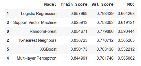
As we can see, our best candidate is the Logistic Regression model.
Fine-Tuning and Additional Improvements
But can we make any additional changes to improve our best model yet? A natural follow-up is to fine-tune the model's hyper-parameters to optimize it to the data. Let us do that by using a grid search method to determine the optimal settings for the model. Once again, we will create a helper function to receive a parameters dictionary and find the best combination of values.
def grid_search(estimator, param_grid, X_train, X_test, y_train, y_test):
  tune_model = GridSearchCV(estimator, param_grid=param_grid,
                            cv=3, scoring='roc_auc', n_jobs=-1)
  tune_model.fit(X_train, y_train)

  print(type(estimator))

  print("\nGrid scores on development set:\n")

  means = tune_model.cv_results_['mean_test_score']
  stds = tune_model.cv_results_['std_test_score']

  print("%0.3f (+/-%0.03f) for %r\n" %
        (means[tune_model.best_index_], stds[tune_model.best_index_] * 2,
        tune_model.cv_results_['params'][tune_model.best_index_]))

  print("Detailed classification report:\n")
  y_pred = tune_model.predict(X_test)

  print(classification_report(y_test, y_pred, target_names=['Died', 'Survived']))

  return tune_model.best_estimator_
selected_estimator = grid_search(selected_estimator, logistic_grid, X_train,
                                 X_validate, y_train, y_validate)

# Grid scores on development set:

# 0.860 (+/-0.075) for {'C': 1, 'dual': False, 'penalty': 'l1',
# 'solver': 'liblinear', 'tol': 0.0001}
Predicting the Outcome
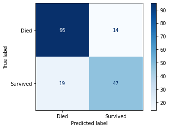
We will generate the predictions for the validation set with the helper method cross_val_predict. And to calculate our final score, we will use the cross_val_score, using accuracy as the scoring metric. Using cross-validation on both, we will test the results with all ten-fold groups used for training. In the end, we got a final result of approximately 82% accuracy, which is pretty reasonable.
y_pred = cross_val_predict(selected_estimator, X_validate, y_validate, cv=kfold)
final_score = cross_val_score(selected_estimator, X_validate, y_validate,
                              scoring='accuracy', cv=kfold)

print(final_score.mean())
# 0.8163398692810457

# Confusion matrix for the Selected Model
plot_confusion_matrix(selected_estimator, X_validate, y_validate,
                      display_labels=['Died', 'Survived'], cmap='Blues')
Optionally we can take the test data and use our model to make the predictions and submit those predictions to the ongoing Kaggle competition. In that case, do not forget to use all the data available (the train and validation sets) to train the final model. I remember making this mistake, where I would forget to use some portion of the data to fit the final model.
Final Thoughts
From this point, there is still a lot of room for improving this work. Some possible options to try can be:
- Test other cross-validation strategies to find the optimal parameters to train our models
- Try out different types of classifiers
- Perform more advanced feature engineering
- Experiment with other techniques like stacking different classifiers and voting mechanisms
- Use Deep Learning models for different architectures.
I keep a GitHub repository where I have my experiments. You can find more details about this project over there.
Thank you for taking the time to read. You can follow me on Twitter, where I share my learning journey. I talk about Data Science, Machine Learning, among other topics I am interested in.